WCET Analysis: The Annotation Language Challenge

The Annotation Language Challenge was proposed at the 7th International Workshop on Worst-Case Execution Time Analysis (WCET 2007) in Pisa, Italy. In this paper we argued that a common annotation language for WCET analysis would be an important step for the WCET community. However, designing such an annotation language is not a simple task. One important step is to create a taxonomy of features the community would want to see in such a language. Our findings are summarised in a paper presented at the 8th Int'l Workshop on WCET analysis (WCET 2008) in Prague, Czech Republic. To further advance the discussion of the topic we have created this web page to reflect our current state of research and future developments of annotation languages.

How to contribute

We would welcome feedback and contributions from the community. If you have any suggestions, please contact us at contact@costa.tuwien.ac.at.

1  Why a Common WCET Annotation Language?

The situation for WCET analysis is very heterogeneous. Within the real-time community it is a well known fact that manual annotations are needed to assist non-perfect analyses. Various tools exist providing different levels of sophistication [17]. However, as the WCET Tool Challenge [6] has shown, few tools share the same target hardware, analysis method or annotation language.

While a multitude of targets is beneficial and a diversity in tools and methods is favorable, a common annotation language is required for an accepted set of benchmarks in order to evaluate the various tools and methods. Still, as a direct consequence of the first WCET Tool Challenge a set of accepted benchmarks has already been collected, without such annotation support.

To enable common annotations within these benchmarks, the WCET Annotation Language Challenge [11] has formulated the need for a common annotation language. This language is a means of specifying the problem-inherent information in a tool- and methodology-independent way, supporting, e.g., static analysis equally well as measurement-based methods, thus allowing the combination of their results. It must also be expressive enough to master the difficult task of providing annotations at the source level, which is the natural specification level, as well as supporting the annotation of binary or object code, if the source code is not available, e.g., for closed sources like operating systems or libraries.

Therefore, a common language may allow the tool developers to concentrate on their analysis methods, creating interchangeable building blocks within the timing analysis framework, as intended by ARTIST2 [9]. By using this common annotation format as a common interface, tools can evaluate the same set of sources for a fair comparison of performance and may exchange analysis results to synergetically supplement each other. The steps of manual annotation, automatic annotation and timing analysis can be repeated, thus iteratively refining the analysis results.

All this should foster common established practices and may, eventually, lead to standardization, resulting in a broader dissemination of WCET analysis throughout research and industry.

2  Basic Concepts

2.1  Definitions

Flow Constraints:

We define flow constraints to be any information about the control or data flow of a program code. Data flow, however, is not only meant in the sense of def-use chains, but, for example, variable-value ranges at program locations. Typical examples of flow constraints are loop bounds or descriptions of (in)feasible paths.

Timing Constraints:

We define timing constraints to be any information that is introduced in order to describe the search space of the WCET analysis.

Because control and data flow represent the basis for the WCET analysis, the flow constraints of a program are always part of the timing constraints. An example of a timing constraint not being a flow constraint is the specification of access times of different memory areas.

Constraints versus Annotations:

We distinguish between the timing constraints and the timing annotation of program code. The timing constraints are the information per se and the timing annotation is the linkage of the timing constraints with the program code.

There are different possibilities of how to annotate the program code with timing constraints. One possibility to annotate the program is to write the timing constraints directly into the source code, either as native statements of the programming language or as special comments. It is also possible to place timing constraints in a separate file, if the source code may not be changed.

If a programmer has to annotate the program modules at different representation levels a common syntax for the different representation levels would be especially beneficial and useful.

2.2  Layers

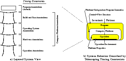
The WCET of a program cannot be determined precisely without knowing information about the target-computer platform on which the program will be used. The computer platform of a program includes, for example, the development tools, the operating system, the hardware, and the application environment. Naturally, the computer platform is sliced into layers to benefit from the independence of different parts that constitute the computer platform. For example, the operating system is an optional layer that may be placed on top of the hardware layer, and again, the layer of the development tool chain may be on top of the operating system.

These layers are the key to the reuse of timing annotations in case a layer is changed. For example, if we change the processor type (hardware layer) but still use exactly the same code binary, any timing constraints describing the behavior of the build-and-run layer can still be reused, if it does not specify explicit times.

A prerequisite for the smooth replacement of layers is that each annotation has a layer specified in its definition. A layer is replaced by disabling the current instance of the layer and enabling another one as input for the analysis.

Note that the layers are not fixed, but rather open for extensions. For example, if an operating system delivered in binary form has different absolute times specified for different processor types, it does make sense to specify them in a combined OS/HW layer besides the other OS and HW layers.

2.3  Validity of Timing Constraints (Timing Invariants vs. Fictions)

The goal of WCET analysis is to calculate a precise WCET bound. However, the developer might also be interested in experimenting with the timing constraints to analyze changes of the program behavior, e.g., to tune the system. For example, the developer might specify a fictive loop bound to determine the influence of the loop on the overall timing. As another example, the developer might want to test an absolute time bound for a code section independently of the real execution time. In both scenarios, timing constraints are not necessarily used to describe a superset of the real program behavior.

In WCET analysis research, program annotations are typically assumed to describe a superset of the possible system behavior, i.e., system invariants. We extend this annotation concept to information that does not have to be a superset of the system behavior. We call all timing constraints that describe a superset of the possible system behavior timing invariants. In contrast, we introduce timing fictions as arbitrary timing constraints the user might want to use for experimenting with the timing behavior of the system. We add a flag to each timing annotation to mark it either as a timing invariant or a timing fiction.

The intention of introducing timing fictions is not to foster its use for WCET analysis, because timing fictions may cause an underestimation of the WCET. But in case that a developer wants to experiment with the sensitivity of the timing behavior, then it is an additional safety feature if the user is able to explicitly mark such timing constraints as timing fictions and has to enable them explicitly to be included in the analysis.

Definition 1.

(Timing Invariant): A timing constraint C is a timing invariant at its associated annotation layer L, iff for all possible systems that use annotation layer L, it holds that for all possible initial system states the system execution fulfills the timing constraint C. If a timing constraint is associated with more than one layer, then the condition has to hold for all possible systems that use all of its associated layers.

Definition 2.

(Timing Fiction): If a timing constraint C is not a timing invariant at its associated annotation layer, then it is a timing fiction.

In the case that timing invariants and timing fictions are in conflict, the semantics of timing fictions is to override conflicting timing invariants. Whenever a timing invariant is overridden due to a timing fiction, the WCET analysis tool should give a log entry to the user.

The following provides examples of timing invariants and timing fictions:

void f (int a, char[] b)
{
  int i;
  a = a % 20;
  for (i=0; i<a; i++) //loop1
  {
    if (i%2 == 0)
      b[i] = a; //m1
    else
      b[i] = 0; //m2
  }
}

In the timing fiction example with loop bound LB(loop1)=40… 40, an IPET-based WCET analysis tool typically transforms the program structure into flow equations and the fictive loop bound is transformed into a flow constraint. In this case, the timing fiction redefines the execution count of control-flow edges in the final WCET calculation.

2.4  Checking of Invariants

Manual annotations are potentially error-prone and may yield incorrect WCET estimates. In the case that timing constraints originate from the operation environment it is, however, possible to "lift" operation environment information to the program layer, e.g., by inserting range checks and similar assertions wherever appropriate.

int count = read_from_sensor();
while (count >= 0) {
  count--;
  ...
  

int count = read_from_sensor();
if(count < 48) {
  while (count >= 0) {
    count--;
    ...
  } else {
    error();
  }

  

As a result of lifting annotations to the program layer, the resulting program becomes a specialized instance of the original program. Because the assertions allow the compiler to perform additional optimizations, the specialized program can also have better performance than the original program. These kinds of assertions can easily be generated by an automatic tool and could be valuable for diagnosis and testing of annotations. An example of using runtime checks with special support by the compiler is Modula/R: the Modula/R compiler optionally generates for each source-code location that is referenced by a timing constraint a separate counter variable where an exception is raised at runtime if their specified bound is exceeded [16].

3  Ingredients of the WCET Annotation Language

In the following we describe essential ingredients for a WCET annotation language. The different timing constraints are described at a conceptual level without focusing on the concrete syntax of an annotation language. We use ANSI C code examples to illustrate the usefulness of the different timing constraints. The definition of a concrete syntax is beyond the scope of this paper. We propose the following categories of ingredients, which are detailed in the rest of this section:

1. Annotation Categorization
2. Program-Specific Annotations
3. Addressable Units
4. Control Flow Information
5. Hardware-Specific Annotations

1. []Annotation Categorization
   We define attributes for timing constraints to categorize and group them. These categorization attributes help to organize, check, and maintain timing annotations. Supporting the maintenance of timing annotations is a very important aspect to improve the correctness of timing constraints. For example, if a user writes an annotation with speculative constraints just for testing the influence on the timing behavior of the system, there is the potential danger that he/she forgets to remove such an annotation from the program later on. Further, whenever code is reused or parts of the computer platform are changed, it is necessary to identify those annotations that have to be checked or adapted. The categorizations 1(a), 1(b), and 1(c) are orthogonal categorizations, but their joint use is intended.
   1. Annotation Layer
      Each timing constraint has associated an annotation layer to describe its validity. As described in Section 2.2, the WCET of a program depends on its computer platform. The computer platform is typically divided into several layers, allowing the customization of the system at each layer. As shown in Figure 1(b) we propose to support the specification of at least the following three annotation layers:

      Program Layer:

      If an annotation belongs solely to the program layer, the timing constraint is assumed to be platform-independent. Here it is important to note that in programming languages like C or C++ the functional behavior is not fully platform-independent, i.e., some timing constraints about the control flow may already belong to the computer-platform layer.

      Computer-Platform Layer:

      The computer platform of a program includes everything necessary to execute the program. If a finer granularity is needed, the platform may be divided into different layers, like, for example, the build and run environment, the operating system, any middleware, and also the hardware (as shown in Figure 1(b).a).

      For example, the cache geometry and the cache miss penalty may be specified at the hardware layer. As another example, knowing the attached flash memory device, one may specify the time needed for the completion of a write access.

      Figure 1(b) also shows the difference between the orthogonal layers and the interface, a platform presents to a stack of layers. In Figure 1(b).a we see the different annotation layers, including the computer-platform layers, each of them clearly separated from the others. Please note the difference between a computer-platform layer (a name of an annotation layer) and a platform (as described in the MDA [13] of the OMG). In contrast to an annotation layer, a platform subsumes all the annotation layers below it. The platform can also be seen as an interface that comprises the information belonging to all annotation layers below it. Thus, as shown in Figure 1(b).b, the system behavior influenced by each interface contains the behavior of all annotation layers below it.

      Operation Layer:

      The operation layer describes the usage of the computer system, i.e., how the environment of the system is configured and how the environment behaves.

      For example, timing constraints at the application layer may describe that the computer system is connected to three sensors, implying that a loop in the software to poll these sensors will iterate exactly three times.

      
      
      The program-, computer-platform- and operation-layers are examples, only. Based on the specific system architecture, the user may refine the layering to further annotation layers. It can also happen that a timing constraint is associated to multiple annotation layers. However, whenever possible, it is advised to split such constraints into multiple constraints where each constraint belongs only to a single annotation layer. Note that the layer stack suggested by Figure 1(b).a is not mandatory; layers may be also placed horizontally. But the important point is that the different layers should be orthogonal, so that it is relatively easy in the system to exchange a layer and its specific timing annotations.

      For timing constraints that refer to annotation layers other than the program layer, or timing constraints that represent fictions, more care has to be taken to ensure their intended use. For example, a loop bound may be tighter using information from the operation layer, as opposed to using only information from the program layer. Constraints refined with information from the operation layer are associated naturally also to the operation layer.

   2. Annotation Class
      The annotation class is an attribute to describe the validity of timing constraints. As described in Section 2.3, besides the timing invariants we also introduce timing fictions as additional class of timing constraints. Each timing constraint should therefore contain a flag that indicates its class.

      Invariants:

      Invariants are used to explicitly annotate information which is assumed to be valid with respect to the concrete semantics of the associated annotation layer.

      Fictions:

      Timing fictions are used to provide fictive timing constraints to experiment with the sensitivity of a system's timing behavior.

      ---

      
      Layered Timing Constraints

      ---

      The criterion of whether a timing constraint is an invariant (and not a fiction) is not only whether it holds for each possible input data on the program code. This is because, as shown in Figure 1(b).b, the system can be annotated at different layers (layers are described by the timing-constraint attributes 1(a)).

      For example, if a timing constraint describes properties of the computer-platform layer, we have to look at the concrete computer platform to decide whether this timing constraint is a timing invariant or a timing fiction.

   3. Annotation Group
      The grouping mechanism allows for different WCET evaluations. For each annotation group a separate WCET calculation with its own set of timing constraints can be conducted.

      There are several reasons why one might use different sets of timing constraints. For example, one might want to use and annotate different scenarios at the operation layer, or different tool chains at the computer-platform layer, etc. Timing fictions can be organized in groups as well to ensure their selective and correct use.

      The grouping mechanism allows us to give each timing constraint membership to multiple groups. A group is a symbolic name together with a description field. There is no special semantics behind the groups: their intended meaning has to be described in their description fields. With the grouping mechanism one can specify which timing constraints will be used together for WCET analysis. Hierarchical definitions of groups are supported by specification of an optional list of nested groups.

      Timing constraints that are invariants at the program layer are relatively easy to maintain. They can be checked directly against the source code and they only have to be changed if the program code changes. They remain valid if the computer platform changes.

2. Program-Specific Annotations
   We define program-specific annotations as timing constraints that directly describe the control and data flow of a program.
   1. Loop Bounds
      Loop bounds comprise the minimal timing constraints at the program layer that are necessary to estimate the WCET of a program. For this reason, they were the first type of annotation that was introduced in the short history of WCET annotation languages [11].

      Although loop bounds can always be expressed through linear flow constraints, there are practical reasons to allow loop bounds to be specified in a specialized and more compact notation. To maintain a tight execution count estimate after certain loop optimizations, it is desirable to specify lower loop bounds directly.

      int i; for (i = 0; i < n; ++i) { process(g[n]); }	Here, the loop bound depends on the value of variable n. Static interprocedural program analysis over the whole program may find that the possible value of n at the beginning of the loop is 3...10, resulting in a lower loop bound of 3 and an upper loop bound of 10.

   2. Recursion Bounds
      When a recursion is bounded, time and stack size requirements are also bounded using this recursion depth. If such conditions cannot be established by analysis, user annotations can supply the required data. In analogy to the earlier work on loop-bounds [1], Blieberger and Lieger established the conditions necessary for establishing upper bounds for stack space and time requirements of directly recursive functions. They also generalize the approach to indirectly recursive functions [2]. Recursion depth annotations are also used by Ferdinand et al. [4].

      unsigned fac(unsigned n) { if (n == 0) return 1; else return n*fac(n-1); }	The most precise recursion bound of procedure fac is the maximum value of input variable n. If a static program analysis finds fac always to be called with n ≤ 10, then 10 is the most precise recursion bound.

   3. Linear Flow Constraints
      Linear flow constraints are the basis for IPET-based WCET calculation methods. In the course of the calculation, all other program-specific constraints and control-flow constraints will eventually get translated into linear flow constraints. While flow constraints have a very high expressiveness, they are not necessarily as easy to write as, e.g., loop bounds, which is one of the reasons for allowing multiple ways of annotating the same flow constraint.

      Linear flow constraints are used to express a relationship between certain reference points in the control flow graph (CFG) of a program. From the perspective of the source language this necessitates the introduction of auxiliary annotations like markers (to obtain a reference point) and scopes (to restrict the lexical validity of a constraint). The constraints themselves are usually called restrictions.

      for (i = 0; i < n; ++i) { for (j = i; j >= 0; --j) { stmt1; } }	We assume that the execution count of the entry of the outer loop is labeled as m0 and the execution count of the inner loop's body is labeled as m1. Then, the linear flow constraint "m1 ≤ n·(n−1)/2· m0" can be used to provide refined information about the execution count of the loop nest.

   4. Variable-Value Restrictions
      Variable-value restrictions describe data-flow and are thus not a direct control-flow restriction. Variable-value restrictions can be transformed into an explicit control-flow restriction by a program analysis tool.

      if (i < 72) { stmt1; ...	Directly before stmt1 the value of i is confined by imin ≤ i < 72, where imin is the smallest possible value of the data type of i.

   5. Summaries of External Functions
      Often, software libraries are distributed as binaries and without any source code. In these cases, the library manufacturer could provide summaries of the library functions that contain the missing information that is necessary to analyze programs that use the library. A summary of a function may contain side effects (list of modified items) or value ranges of the returned values. A function summary may still be useful, even when the source code is available, e.g., for hard-to-analyze facts.

      int signum(int x);	The subroutine signum is assumed to be pure and returns −1,0 or +1. Thus we can annotate that the set of objects modified by this subroutine is empty, and the value returned by the subroutine is always from within [−1,1].

3. Addressable Units
   Addressable units of an annotation language are those that can be associated with timing constraints. The more language constructs and levels of abstraction can be addressed, the more fine-grained timing constraints can be specified. Examples of how to address different units of the program layer are given in [8]. In this section we list all language constructs that we consider relevant for being annotated with timing constraints.
   1. Control-Flow Addressable Units
      Conceptually, WCET annotations typically express relationships between nodes, edges and paths of the CFG. If the paths between functions are included in the graph as well then we call this graph an interprocedural control flow graph (ICFG) [15]. Although the ICFG is implicitly defined by the program structure, it is not generally visible and will be generated ad hoc by the compiler. The annotation language therefore faces the problem to address entities inside a graph that have no standardized explicit representation.

      We thus propose the following addressable units of the ICFG based on the program source code:

      1. Basic Blocks
         A basic block is a code sequence with single entry and single exit point. For timing analysis it is relevant that execution passes a basic block's entry point as often as its exit point. Thus, instead of annotating the basic block, any location within the basic block can hold the block annotation.
      2. Edges
         Edges in the CFG, however, do not necessarily have a direct counterpart in the program because they are implicitly defined by the semantics of the respective language construct.

         To circumvent this problem we introduce a set of reserved edge-names for each control flow construct of the source language. For example, considering some constructs of the C language, such names could include TrueEdge_if, FalseEdge_if and BackEdge_while. Such names allow a user to associate timing constraints with specific edges of the respective CFG for a given language construct.

      3. Subgraphs
         Subgraphs of the ICFG can be addressed and thus annotated. For example, an annotation can be associated with an entire function, or with a statement containing several function calls, or some nested loops.

      
      
      To handle control flow inside expressions, such as function calls and short-circuit evaluation, it is necessary to normalize the program first. In this step short-circuit evaluation will be lowered into nested if-statements and function calls are extracted from expressions. For the addressing of subexpressions, a mapping between the normalized code and the original code must be maintained.

   2. Loop Contexts
      For all kinds of loops it may be of interest to annotate specific iterations separately, or to exclude specific iterations, i.e. annotate all but these specific iterations. The most prominent example is that the first (few) iteration(s) may be very different from the following ones due to cache effects.

      for (int i = 0; i < n; ++i) for (int j = 0; j < d; ++j) a[i][j] *= v[j];	Due to the "warming-up" of the cache, the first iteration could show a different behavior than the subsequent iterations.

   3. Call Contexts
      As different call sites are bound to present different preconditions for a function e.g. input values, separate annotation of these different call contexts must be possible.

      void g() { f(50); } int f(int i) { while (--i >= 0) { ... }	The loop bound in function f depends on the value of input variable i. Thus, as a context-dependent flow constraint we can write that the upper loop bound is 50 when f() is directly called by g().

   4. Values of Input Variables
      If a function behaves significantly different depending on the possible values of an input parameter, it can be useful to provide different sets of annotations for each case. This kind of annotation was first introduced with Spark Ada [14] and was called "modes".

      int f(struct data *x) { if (x == NULL) return NULL; ... }	The function may behave completely different depending on whether the input variable x is NULL or not: e.g. whenever x==NULL, the function returns immediately.

   5. Explicit Enumeration of (In)feasible Paths
      In path-based approaches [3, , 14, ], explicit knowledge of the feasibility of paths can be incorporated into the analysis process.

      void worker() { init(); while (cond) process(); } void process() { if (!initialized) init(); ...	In this example, function init() is never called from function process(), if process() itself is called from function worker(). We can thus annotate that there is no path worker→process→init.

   6. The Goto Statement
      The goto statement allows to introduce edges of non-structured control flow. If the target of a goto statement is statically known, it is not necessary to introduce any special annotations to specifically address a goto statement in the CFG; the containing basic block can be used equivalently. If the target address of a goto is not statically known, it makes sense to annotate possible jump targets as described in paragraph 4(c). The break, continue and return statements are specialized (better-behaved) instances of the goto statement in that their branch target is further restricted from function scope to the current control scope. This can be exploited by better analysis, but from the annotation standpoint there is not much difference to the goto except that there is less need for an annotation, when the analysis is easier.
4. Control-Flow Constraints
   The CFG is a valuable abstraction level that can be refined in various ways to improve the precision of the analysis. This is to aid the automatic CFG generation within the tools by additional information that is not available within the program itself.
   1. Unreachable Code
      This is a program-specific annotation, which has been used by Heckmann and Ferdinand [7]. Unreachable code could as well be specified by linear flow constraints. Having a specific mechanism however makes the intention of the user explicit.
   2. Predicate Evaluation
      Closely related to the above case, annotations of predicate evaluations were also introduced by Heckmann and Ferdinand [7]. These kind of annotations describe for conditions/decisions whether they will always evaluate to True or False.
   3. Control-Flow Reconstruction
      Introduced by Ferdinand et al. [5], and further elaborated by Kirner and Puschner [12], the CFG Reconstruction Annotations are used as guidelines for the analysis tool to construct the control flow graph (CFG) of a program. Without these annotations it may not be possible to construct the CFG from the binary or object code of a program.

      On one hand, annotations are used for the construction of syntactical hierarchies within the CFG, i.e., to identify certain control-flow structures like loops or function calls. For example, a compiler might emit ordinary branch instructions instead of specific instructions for function calls or returns. In such cases it might be required to annotate a branch instruction whether it is a call or return instruction.

      The high-level programming language features that can lead to code that is difficult to analyze locally are: function-pointer calls, virtual-method calls, and returns as well as indirect conditional control-flow transfer like computed goto or switch statements or transformation results obtained from combining conditional control flow with ordinary or indirect calls or returns.

      void process((void)(int*) func, int *data) { (*func)(data); }	In this code, it might be known that the target of function pointer func points either to (void)reset(int*) or to (void)iterate(int*).

      A work-around that sometimes helps avoiding code annotations is to match code patterns generated by a specific version of a compiler. However, such a "hack" cannot cover all situations and may also have the risk of incorrect classifications, for example, if a different version of the compiler is used.

      On the other hand, annotations may be needed for the construction of the CFG itself. This may be the case for branch instructions where the address of the branch target is calculated dynamically. Of course, static program analysis may identify a precise set of potential branch targets for those cases where the branch target is calculated locally. In contrast, if the static program analysis completely fails to bind the branch target, it has to be assumed that the branch potentially branches to each instruction in the code, which obviously is too pessimistic in order to compute a useful WCET bound. In such a case, code annotations are required that describe the possible set of branch targets.

      
      

      The following list summarizes examples of code annotations derived from aiT [5, 7]: instruction <addr> calls <target-list>; instruction <addr> branches to <target-list>; instruction <addr> is a return; snippet <addr> is never executed; instruction <addr> is entered with <state>; Note that these annotations must not be linked to a specific instruction type, since an optimizing compiler may combine or change instructions, but the annotation needs to stay.

5. Hardware-Specific Annotations
   For a realistic modeling of the execution behavior of a program, an annotation language also needs mechanisms to describe the behavior of the underlying hardware. Many of these annotations are supported by industrial timing analyzers like aiT [7].

   Since some hardware-specific annotations are associated to the hardware layer only, they are independent from the program layer and can thus be easily reused for multiple programs running on the same embedded platform. It can thus make sense not to annotate this information to program code, but rather gather it in a common location so that it can be combined with the annotations of more than one program.

   Examples of such basic hardware data to be kept separate from the program annotations are:

   Instruction timing: The general timing information of instructions has to be maintained separate from the program.

   Clock rate: The analysis must be able to convert clock ticks to absolute times when computing the WCET, and vice versa for absolute-time specification annotations.

   Access times for ROM, internal and external RAM: It would be tedious and cumbersome to specify these times at each of the various read and write operations.

   Memory map: As the memory map binds memory access times to a multitude of memory access operations, the information that is available to the linker can, when supplied to the timing analysis, largely reduce the annotation effort for the program.

   Hardware implementation details that hold on the program as a whole, and cannot be tied to a single specific program location, also need to be specified separately. Caches or jump prediction details are examples.

   It is not always obvious where to draw the borderline between hardware-specific annotations and information that is better managed by the analysis tool. The following items are examples of timing constraints that are reasonably expressed as timing annotations.

   1. Memory and Memory Accesses
      The temporal behavior of memory accesses depends on the characteristics of the memory. Embedded systems typically use different types of memory depending on the access frequency and access pattern. It is thus necessary to specify the following characteristics:
      • address range of read operations
      • address range of write operations
      • writeable memory area (RAM) and read-only memory area (ROM)
      • data and code regions
      • access time of specific memory regions (in cycles or ms)
   2. Absolute Time Bounds
      Providing a means for absolute time bounds allows to specify the maximum and minimum execution time of a fraction of code. Such a feature can be found in wcetC [10], for example.

      char poll() { volatile char io_port; while (io_port != 0) /* wait */ ; }	It could be an invariant of the hardware platform that the execution time of the subroutine poll() (busy waiting) is always between 30 and 100µ s.

Acknowledgments
We would like to thank Niklas Holsti from Tidorum Ltd for his valuable comments on this paper.

References

[1]

Johann Blieberger. Discrete loops and worst case performance. Computer Languages, 20(3):193–212, 1994.

[2]

Johann Blieberger. Real-time properties of indirect recursive procedures. Inf. Comput., 171(2):156–182, 2001.

[3]

Roderick Chapman, Alan Burns, and Andy Wellings. Combining static worst-case timing analysis and program proof. Real-Time Systems, 11(2):145–171, 1996.

[4]

Christian Ferdinand, Reinhold Heckmann, Marc Langenbach, Florian Martin, Michael Schmidt, Henrik Theiling, Stephan Thesing, and Reinhard Wilhelm. Reliable and precise WCET determination for a real-life processor. In Proc. of the 1st Int'l Workshop on Embedded Software (EMSOFT 2001), Tahoe City, CA, USA, Oct. 2001.

[5]

Christian Ferdinand, Reinhold Heckmann, and Henrik Theiling. Convenient user annotations for a WCET tool. In Proc. 3rd International Workshop on Worst-Case Execution Time Analysis, pages 17–20, Porto, Portugal, July 2003.

[6]

Jan Gustafsson. The WCET tool challenge 2006. In Preliminary Proc. 2nd Int. IEEE Symposium on Leveraging Applications of Formal Methods, Verification and Validation, pages 248 – 249, Paphos, Cyprus, November 2006.

[7]

Reinhold Heckmann and Christian Ferdinand. Combining automatic analysis and user annotations for successful worst-case execution time prediction. In Embedded World 2005 Conference, Nürnberg, Germany, Feb. 2005.

[8]

Niklas Holsti. Bound-T Assertion Language. Tidorum Ltd, Helsinki, Finland, 6.2 edition, Feb. 2008. online available at: http://www.tidorum.fi/bound-t/assertion-lang.pdf.

[9]

IST-004527. The ARTIST2 Network of Excellence on Embedded Systems Design. http://www.artist-embedded.org/, September 1st 2004 - August 31st 2008. ARTIST2 is funded by the European Commission within FP6.

[10]

Raimund Kirner. The programming language wcetC. Technical report, Technische Universität Wien, Institut für Technische Informatik, Treitlstr. 1-3/182-1, 1040 Vienna, Austria, 2002.

[11]

Raimund Kirner, Jens Knoop, Adrian Prantl, Markus Schordan, and Ingomar Wenzel. WCET analysis: The annotation language challenge. In Proc. 7th International Workshop on Worst-Case Execution Time Analysis, Pisa, Italy, July 2007.

[12]

Raimund Kirner and Peter Puschner. Classification of code annotations and discussion of compiler-support for worst-case execution time analysis. In Proc. 5th International Workshop on Worst-Case Execution Time Analysis, Palma, Spain, July 2005.

[13]

Object Management Group. MDA Guide, version 1.0.1 edition, June 2003. document number: omg/2003-06-01.

[14]

Chang Y. Park. Predicting program execution times by analyzing static and dynamic program paths. Real-Time Systems, 5(1):31–62, 1993.

[15]

Micha Sharir and Amir Pnueli. Two approaches to inter-procedural data-flow analysis. In Steven S. Muchnik and Neil D. Jones, editors, Program Flow Analysis: Theory and Applications. Prentice-Hall, 1981. ISBN:0137296819.

[16]

Alexander Vrchoticky. Modula/R - Language Definition. Technical report, Technische Universität Wien, Institut für Technische Informatik, Treitlstr. 1-3/182-1, 1040 Vienna, Austria, Mar. 1992.

[17]

Reinhard Wilhelm, Jakob Engblom, Andreas Ermedahl, Niklas Holsti, Stephan Thesing, David Whalley, Guillem Bernat, Christian Ferdinand, Reinhold Heckman, Tulika Mitra, Frank Mueller, Isabelle Puaut, Peter Puschner, Jan Staschulat, and Per Stenstrom. The worst-case execution time problem - overview of methods and survey of tools. ACM Transactions on Embedded Computing Systems (TECS), 7(3), Apr. 2008.